How to analyse the model output

I assume that you have read the tutorial on how to prepare the input data and run a simulation (see here). In this tutorial, we will analyse the output of the simulation that is stored in the object sol.

import GrasslandTraitSim as sim

using Statistics
using CairoMakie
using Unitful
using RCall # only for functional diversity indices
CairoMakie.activate!()

trait_input = sim.input_traits()
input_obj = sim.validation_input("HEG01");
p = sim.optim_parameter()
sol = sim.solve_prob(; input_obj, p, trait_input);

Biomass

We can look at the simulated biomass:

sol.output.biomass

╭──────────────────────────────────────────────────────────────────────────────╮
│ 6210×1×1×70 DimArray{Unitful.Quantity{Float64, 𝐌 𝐋^-2, Unitful.FreeUnits{(ha^-1, kg), 𝐌 𝐋^-2, nothing}},4} state_biomass │
├──────────────────────────────────────────────────────────────────────── dims ┤
  ↓ time    Sampled{Dates.Date} Dates.Date("2006-01-01"):Dates.Day(1):Dates.Date("2023-01-01") ForwardOrdered Regular Points,
  → x       Sampled{Int64} 1:1 ForwardOrdered Regular Points,
  ↗ y       Sampled{Int64} 1:1 ForwardOrdered Regular Points,
  ⬔ species Sampled{Int64} 1:70 ForwardOrdered Regular Points
└──────────────────────────────────────────────────────────────────────────────┘
[:, :, 1, 1]
 ↓ →                                   1
  2006-01-01    71.4286 kg ha^-1
  2006-01-02    71.3399 kg ha^-1
  2006-01-03    71.2514 kg ha^-1
 ⋮                    
  2022-12-29   0.100067 kg ha^-1
  2022-12-30   0.099876 kg ha^-1
  2022-12-31  0.0996935 kg ha^-1
  2023-01-01  0.0995072 kg ha^-1

The four dimension of the array are: daily time step, patch x dim, patch y dim, and species. For plotting the values with Makie.jl, we have to remove the units with ustrip:

# if we have more than one patch per site, we have to first calculate the mean biomass per site
species_biomass = dropdims(mean(sol.output.biomass; dims = (:x, :y)); dims = (:x, :y))
total_biomass = vec(sum(species_biomass; dims = :species))

fig, _ = lines(sol.simp.output_date_num, ustrip.(total_biomass), color = :darkgreen, linewidth = 2;
      axis = (; ylabel = "Total dry biomass [kg ha⁻¹]",
                xlabel = "Date [year]"))
fig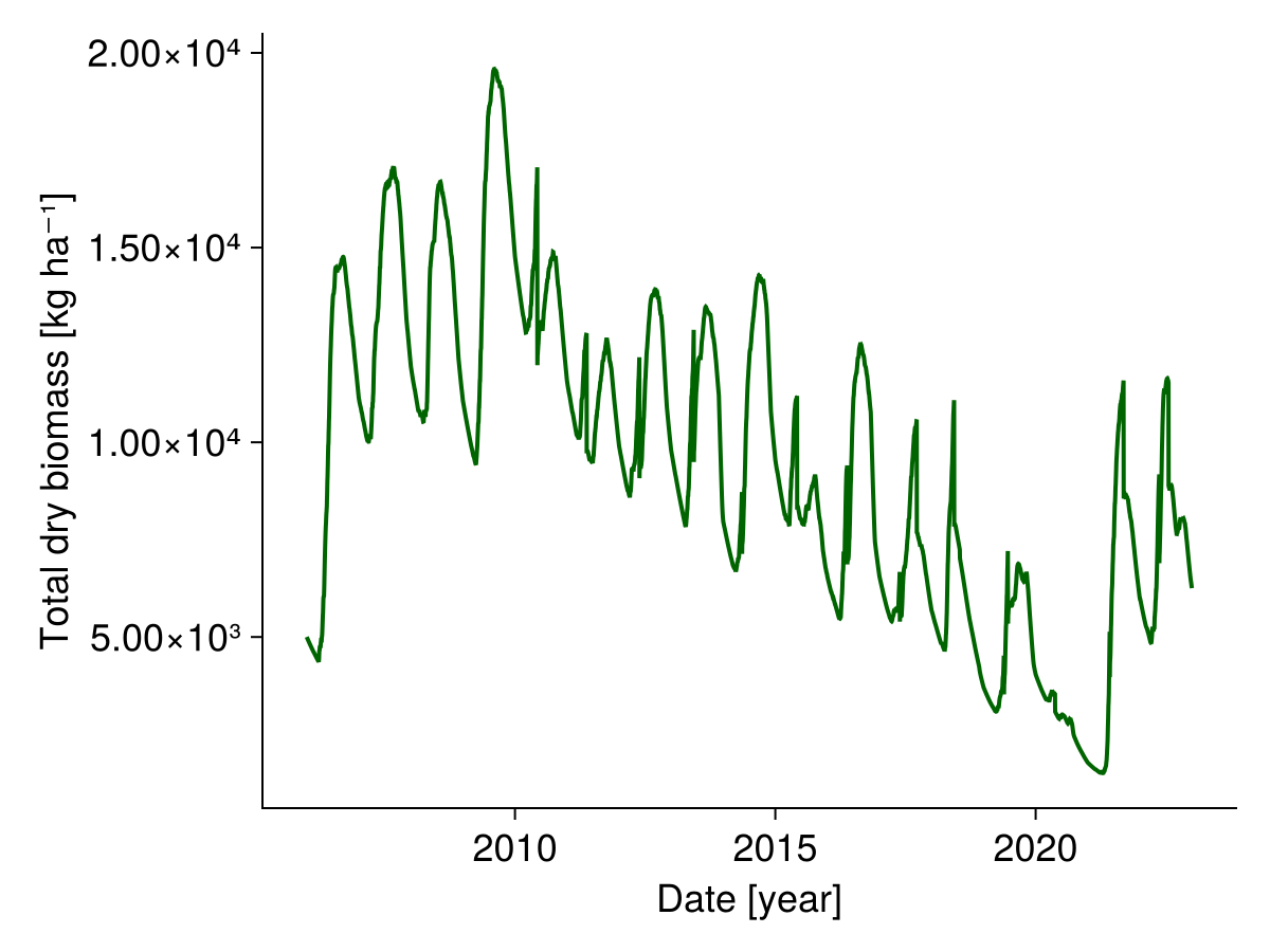

Height of the community

We can also look at the simulated height of each species:

sol.output.height

╭──────────────────────────────────────────────────────────────────────────────╮
│ 6210×1×1×70 DimArray{Unitful.Quantity{Float64, 𝐋, Unitful.FreeUnits{(m,), 𝐋, nothing}},4} state_height │
├──────────────────────────────────────────────────────────────────────── dims ┤
  ↓ time    Sampled{Dates.Date} Dates.Date("2006-01-01"):Dates.Day(1):Dates.Date("2023-01-01") ForwardOrdered Regular Points,
  → x       Sampled{Int64} 1:1 ForwardOrdered Regular Points,
  ↗ y       Sampled{Int64} 1:1 ForwardOrdered Regular Points,
  ⬔ species Sampled{Int64} 1:70 ForwardOrdered Regular Points
└──────────────────────────────────────────────────────────────────────────────┘
[:, :, 1, 1]
 ↓ →                           1
  2006-01-01       0.4 m
  2006-01-02       0.4 m
  2006-01-03       0.4 m
 ⋮                    
  2022-12-29  0.235389 m
  2022-12-30   0.23564 m
  2022-12-31  0.236601 m
  2023-01-01  0.237188 m

We calculate the height of the community by weighting the height of the species by their proportion of biomass on the total biomass:

species_biomass = dropdims(mean(sol.output.biomass; dims = (:x, :y)); dims = (:x, :y))
total_biomass = vec(sum(species_biomass; dims = :species))
species_height = dropdims(mean(sol.output.height; dims = (:x, :y)); dims = (:x, :y))
community_height = vec(sum(species_height .* species_biomass ./ total_biomass; dims = :species))

fig, _ = lines(sol.simp.output_date_num, ustrip.(community_height),
                color = :seagreen, linewidth = 2;
    axis = (; ylabel = "Community height [m]",
                xlabel = "Date [year]"))
fig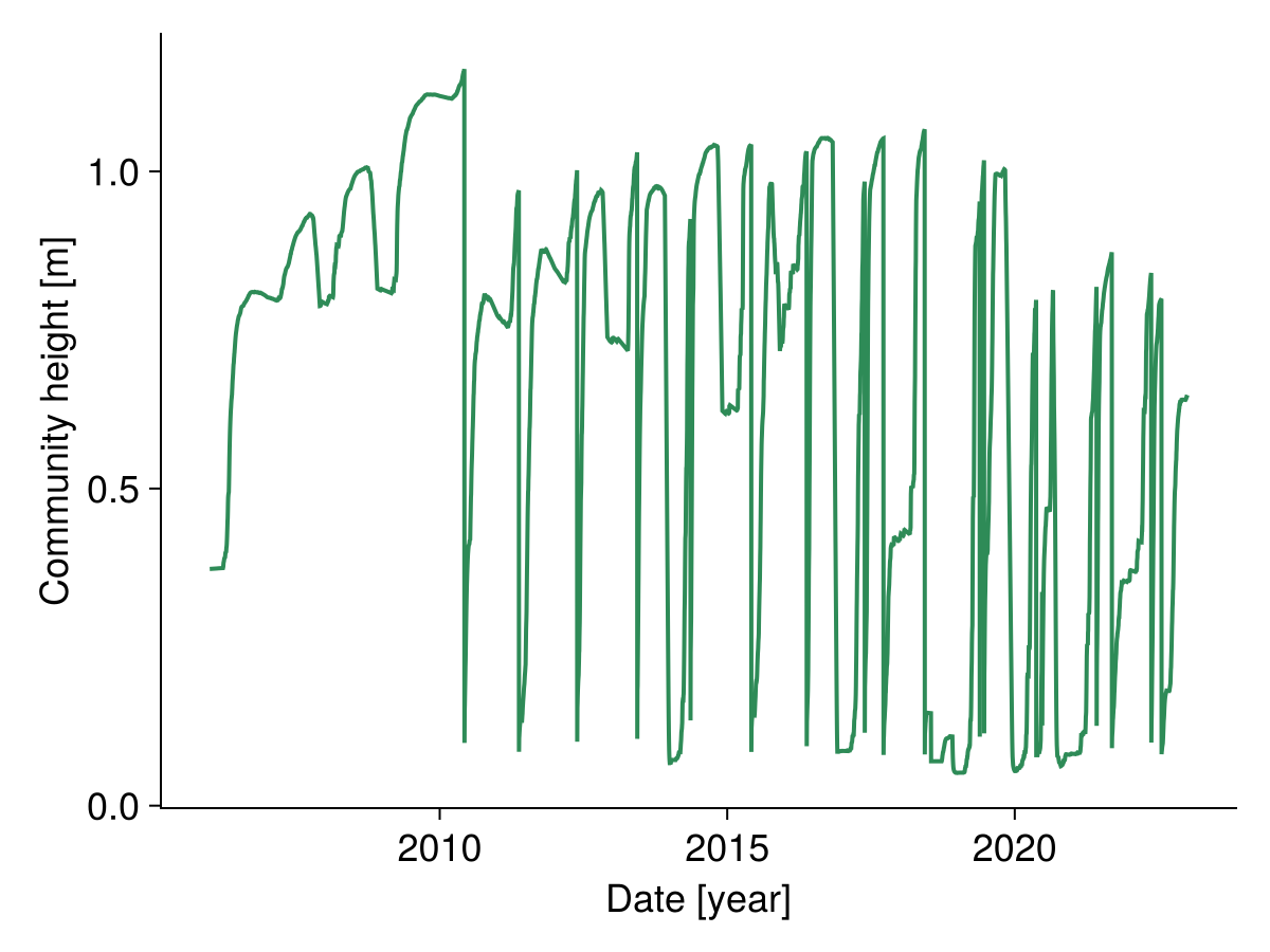

Share of each species

We can look at the share of each species over time:

show code

# colors are assigned according to the specific leaf area (SLA)
color = ustrip.(sol.traits.sla)
colormap = :viridis
colorrange = (minimum(color), maximum(color))
is = sortperm(color)
cmap = cgrad(colormap)
colors = [cmap[(co .- colorrange[1]) ./ (colorrange[2] - colorrange[1])]
          for co in color[is]]

# calculate biomass proportion of each species
biomass_site = dropdims(mean(sol.output.biomass; dims=(:x, :y)); dims = (:x, :y))
biomass_ordered = biomass_site[:, sortperm(color)]
biomass_fraction = biomass_ordered ./ sum(biomass_ordered; dims = :species)
biomass_cumfraction = cumsum(biomass_fraction; dims = 2)

begin
    fig = Figure()
    Axis(fig[1,1]; ylabel = "Relative proportion of biomass of the species",
         xlabel = "Date [year]",
         limits = (sol.simp.output_date_num[1], sol.simp.output_date_num[end], 0, 1))

    for i in 1:sol.simp.nspecies
        ylower = nothing
        if i == 1
            ylower = zeros(size(biomass_cumfraction, 1))
        else
            ylower = biomass_cumfraction[:, i-1]
        end
        yupper = biomass_cumfraction[:, i]

        band!(sol.simp.output_date_num, vec(ylower), vec(yupper);
              color = colors[i])
    end

    Colorbar(fig[1,2]; limits = colorrange, colormap = cmap,
             label = "Specific leaf area [m² g⁻¹]")

    fig
end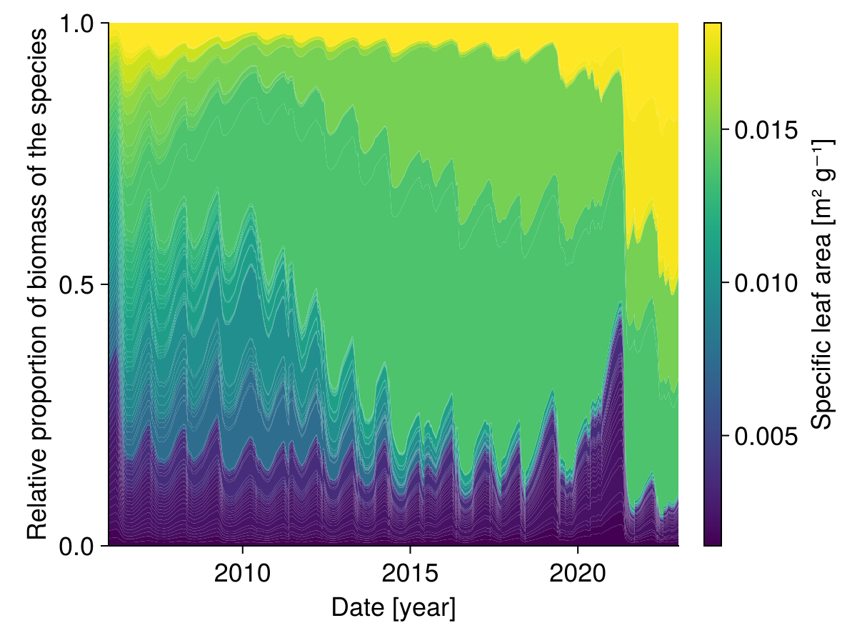

Soil water content

Similarly, we plot the soil water content over time:

# if we have more than one patch per site,
# we have to first calculate the mean soil water content per site
soil_water_per_site = dropdims(mean(sol.output.water; dims = (:x, :y)); dims = (:x, :y))

fig, _ = lines(sol.simp.output_date_num, vec(ustrip.(soil_water_per_site)), color = :blue, linewidth = 2;
      axis = (; ylabel = "Soil water content [mm]", xlabel = "Date [year]"))
fig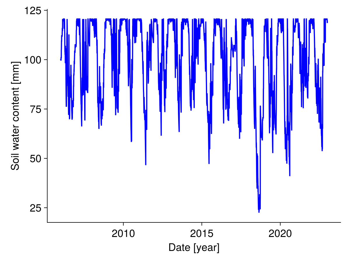

Community weighted mean traits

We can calculate for all traits the community weighted mean over time:

show code

relative_biomass = species_biomass ./ total_biomass
traits = [:maxheight, :sla, :lnc, :rsa, :amc, :abp, :lbp]
trait_names = [
    "Maximum\n height [m]", "Specific leaf\narea [m² g⁻¹]", "Leaf nitrogen \nper leaf mass\n [mg g⁻¹]",
    "Root surface\narea per below\nground biomass\n[m² g⁻¹]", "Arbuscular\n mycorrhizal\n colonisation",
    "Aboveground\nbiomass per total\nbiomass [-]", "Leaf biomass\nper total \nbiomass [-]"]

begin
    fig = Figure(; size = (500, 1000))

    for i in eachindex(traits)
        trait_vals = sol.traits[traits[i]]
        weighted_trait = trait_vals .* relative_biomass'
        cwm_trait = vec(sum(weighted_trait; dims = 1))

        Axis(fig[i, 1];
                xlabel = i == length(traits) ? "Date [year]" : "",
                xticklabelsvisible = i == length(traits) ? true : false,
                ylabel = trait_names[i])
        lines!(sol.simp.output_date_num, ustrip.(cwm_trait);
                color = :black, linewidth = 2)

    end

    [rowgap!(fig.layout, i, 5) for i in 1:length(traits)-1]

    fig
end

Grazed and mown biomass

We can look at the grazed and mown biomass over time:

show code

# total
sum(sol.output.mown)
sum(sol.output.grazed)

# plot the grazed and mown biomass over time
grazed_site = dropdims(mean(sol.output.grazed; dims=(:x, :y, :species)); dims=(:x, :y, :species))
cum_grazed = cumsum(grazed_site)

mown_site = dropdims(mean(sol.output.mown; dims=(:x, :y, :species)); dims=(:x, :y, :species))
cum_mown = cumsum(mown_site)
begin
      fig = Figure()
      Axis(fig[1,1]; ylabel = "Cummulative grazed\nbiomass [kg ha⁻¹]")
      lines!(sol.simp.mean_input_date_num, ustrip.(vec(cum_grazed)), color = :black, linewidth = 2;)
      Axis(fig[2,1]; ylabel = "Cummulative mown\nbiomass [kg ha⁻¹]", xlabel = "Date [year]")
      lines!(sol.simp.mean_input_date_num, ustrip.(vec(cum_mown)), color = :black, linewidth = 2;)
      fig
end

Functional diversity indices

We use the R-package fundiversity to compute the functional diversity indices. We run the R-code from Julia using the Julia package RCall.jl. We assume that species are present if their biomass is larger than 1 kg/ha.

show code

################ Calculate functional diversity in R
function traits_to_matrix(trait_data; std_traits = true)
    trait_names = keys(trait_data)
    ntraits = length(trait_names)
    nspecies = length(trait_data[trait_names[1]])
    m = Matrix{Float64}(undef, nspecies, ntraits)

    for i in eachindex(trait_names)
        tdat = trait_data[trait_names[i]]
        if std_traits
            m[:, i] = (tdat .- mean(tdat)) ./ std(tdat)
        else
            m[:, i] = ustrip.(tdat)
        end
    end

    return m
end

trait_input_wo_lbp = Base.structdiff(trait_input, (; lbp = nothing))

tstep = 100
biomass = sol.output.biomass[1:tstep:end, 1, 1, :]
biomass[biomass .< 1.0u"kg / ha"] .= 0.0u"kg / ha"
biomass_R = ustrip.(biomass.data)
traits_R = traits_to_matrix(trait_input_wo_lbp;)
site_names = string.("time_", 1:size(biomass_R, 1))
species_names = string.("species_", 1:size(biomass_R, 2))

## transfer data to R
@rput species_names site_names traits_R biomass_R

R"""
library(fundiversity)

rownames(traits_R) <- species_names
rownames(biomass_R) <- site_names
colnames(biomass_R) <- species_names

fric_std_R <- fd_fric(traits_R, biomass_R, stand = TRUE)$FRic
fdis_R <- fd_fdis(traits_R, biomass_R)$FDis
fdiv_R <- fd_fdiv(traits_R, biomass_R)$FDiv
feve_R <- fd_feve(traits_R, biomass_R)$FEve
"""

## get results back from R
@rget fric_std_R fdis_R fdiv_R feve_R

begin
    fig = Figure(size = (900, 1200))

    Axis(fig[1, 1]; ylabel = "Number of species", xticks = 2006:2:2022,
         xticklabelsvisible = false, limits = (nothing, nothing, 0, nothing))
    nspecies = sum(biomass .> 0.0u"kg / ha"; dims = :species)
    lines!(sol.simp.output_date_num[1:tstep:end], vec(nspecies);)

    Axis(fig[2, 1]; yscale = identity, xticks = 2006:2:2022, xticklabelsvisible = false,
         ylabel = "Functional richness -\nfraction of possible volume\nto actual trait volume")
    lines!(sol.simp.output_date_num[1:tstep:end], fric_std_R)

    Axis(fig[3, 1]; xticks = 2006:2:2022, xticklabelsvisible = false,
         ylabel = "Functional dispersion -\nweighted distance to\ncommunity weighted mean")
    lines!(sol.simp.output_date_num[1:tstep:end], fdis_R)

    Axis(fig[4, 1]; xticks = 2006:2:2022, xticklabelsvisible = false,
        ylabel = "Functional divergence -\nweighted distance to\ncenter of convex hull")
    lines!(sol.simp.output_date_num[1:tstep:end], fdiv_R)

    Axis(fig[5, 1]; xticks = 2006:2:2022, xticklabelsvisible = true,
        ylabel = "Functional evenness -\n regularity of species on\nminimum spanning tree,\nweighted by abundance")
    lines!(sol.simp.output_date_num[1:tstep:end], feve_R)

    fig
end

Shannon and Simpson diversity

We can calculate the Shannon and Simpson diversity over time:

show code

biomass_site = dropdims(mean(sol.output.biomass; dims = (:x, :y)); dims = (:x, :y))
tend = size(biomass_site, 1)
shannon = Array{Float64}(undef, tend)
simpson = Array{Float64}(undef, tend)
for t in 1:tend
    b1 = biomass_site[t, :]
    b1 = b1[.!iszero.(b1)]
    p1 = b1 ./ sum(b1)
    shannon[t] = -sum(p1 .* log.(p1))
    simpson[t] = 1 - sum(p1 .^ 2)
end

begin
    fig = Figure()
    Axis(fig[1,1]; ylabel = "Shannon index")
    lines!(sol.simp.output_date_num, shannon, color = :black, linewidth = 2;)
    Axis(fig[2,1]; ylabel = "Simpson index", xlabel = "Date [year]")
    lines!(sol.simp.output_date_num, simpson, color = :black, linewidth = 2;)
    fig
end